Reading Arrays

In the previous tutorials we have provided a fair amount of examples on reading/slicing dense and sparse arrays. Specifically, we explained how to slice and retrieve the results. We also showed that when reading sparse arrays you retrieve only results for the non-empty cells, whereas when reading dense arrays TileDB returns special fill values for any empty/non-populated cells. Finally, we demonstrated how to read only a subset of the array attributes, and also that you can even retrieve the coordinates of the result cells in the case of dense arrays.

In this tutorial we will cover a few more important topics on reading, such as reading in different layouts, determining the memory you need to allocate to your buffers that will hold the results, how to retrieve the non-empty domain of your array, and the concept of “incomplete” queries.

Full programs

Program	Links
reading_dense_layouts
reading_sparse_layouts
reading_incomplete
multi_range_subarray

Basic concepts and definitions

Read query layout

You can read from a TileDB array with different layouts (namely row-major, column-major and global order). The row-/column-major layouts are with respect to your defined subarray and may differ from the physical layout of the cells on disk, attributing a lot of flexibility.

Maximum buffer sizes

One great challenge when reading sparse arrays or arrays with variable-length attributes (dense or sparse) is allocating the result buffers to be set to the query. The reason is that it is not possible to know the exact result size and, hence, it is very hard to calculate how much memory you need to allocate to your buffers. TileDB provides a function for computing a good upper bound estimate on the buffer size that can certainly hold the result for a given attribute.

Non-empty domain

TileDB provides a useful function for determining the non-empty domain of your array, i.e., the tightest hyper-rectangle that encompasses the non-empty cells stored in the (dense or sparse) array.

Incomplete queries

In certain cases, you may wish to read a huge slice incrementally. In such scenarios, allocating a huge buffer for the entire result may not be feasible, whereas you may only have a fixed budget for your buffers. TileDB enables you to submit queries on huge slices with a buffer size budget, and notify you about whether your query is completed or not. If it is incomplete, TileDB grants you a partial result, which you can consume and then resume the query, with TileDB incrementally bringing you the next partial results, and so on.

Multi-range subarrays

TileDB allows specifying a “multi-range” subarray, i.e., more than one ranges for each dimension of the subarray. In the general case TileDB processes multi-range subarray queries more efficiently than issuing multiple separate “single-range” subarrays.

Reading in different layouts

TileDB allows you to retrieve the results of a subarray/slicing query in various layouts with repsect to your specified subarray, namely row-major, column-major and global order. You can set the layout for reads as follows.

C++

query.set_layout(TILEDB_ROW_MAJOR); // Can also be TILEDB_COL_MAJOR or TILEDB_GLOBAL_ORDER

Python

data = A.query(attrs=["a"], order=order, coords=True)[1:3, 2:5]

Observe that the read layout in Python is set in argument order using the query syntax. Setting also coords=True allows you to get the coordinates (even in the dense case). Recall that row-major (order='C') is the default layout of the returned numpy array. Setting order='F' (Fortran-order or column-major) will return a numpy array with the same shape as the requested slice, but which internally lays out the values in column-major order. Finally, setting the global order (order='G') always returns a 1D array, since retaining the slice shape is meaningless when the cells are returned in global order (you can see which value corresponds to which cell by explicitly retrieving the coordinates).

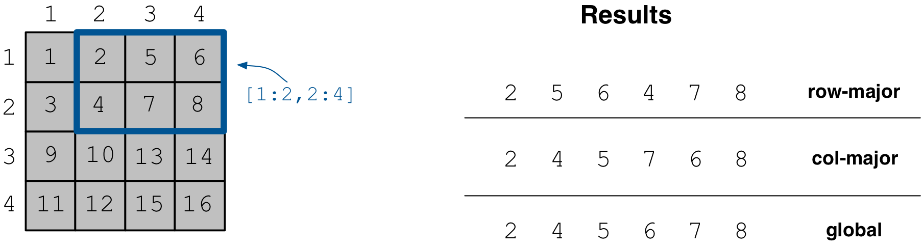
We demonstrate an example of a dense array using code example reading_dense_layouts. The figure below depicts the array contents and the subarray read results for different query layouts. Notice that despite the global ordering of cells in the array, the read results are ordered with respect to the subarray of the query. Note that this is a 4x4 dense array with 2x2 space tiling. The cell values follow the global physical cell order.

Running the program, you get the following output.

C++

$ g++ -std=c++11 reading_dense_layouts.cc -o reading_dense_layouts_cpp -ltiledb
$ ./reading_dense_layouts_cpp row
Non-empty domain: [1,4], [1,4]
Cell (1, 2) has data 2
Cell (1, 3) has data 5
Cell (1, 4) has data 6
Cell (2, 2) has data 4
Cell (2, 3) has data 7
Cell (2, 4) has data 8
$ ./reading_dense_layouts_cpp col
Non-empty domain: [1,4], [1,4]
Cell (1, 2) has data 2
Cell (2, 2) has data 4
Cell (1, 3) has data 5
Cell (2, 3) has data 7
Cell (1, 4) has data 6
Cell (2, 4) has data 8
$ ./reading_dense_layouts_cpp global
Non-empty domain: [1,4], [1,4]
Cell (1, 2) has data 2
Cell (2, 2) has data 4
Cell (1, 3) has data 5
Cell (1, 4) has data 6
Cell (2, 3) has data 7
Cell (2, 4) has data 8

Python

$ python reading_dense_layouts.py row
Non-empty domain: ((1, 4), (1, 4))
Cell (1, 2) has data 2
Cell (1, 3) has data 5
Cell (1, 4) has data 6
Cell (2, 2) has data 4
Cell (2, 3) has data 7
Cell (2, 4) has data 8
$ python reading_dense_layouts.py col
Non-empty domain: ((1, 4), (1, 4))
NOTE: The following result array has col-major layout internally
Cell (1, 2) has data 2
Cell (1, 3) has data 5
Cell (1, 4) has data 6
Cell (2, 2) has data 4
Cell (2, 3) has data 7
Cell (2, 4) has data 8
$ python reading_dense_layouts.py global
Non-empty domain: ((1, 4), (1, 4))
Cell (1, 2) has data 2
Cell (2, 2) has data 4
Cell (1, 3) has data 5
Cell (1, 4) has data 6
Cell (2, 3) has data 7
Cell (2, 4) has data 8

The read query layout specifies how the cell values will be stored in the buffers that will hold the results with respect to your subarray.

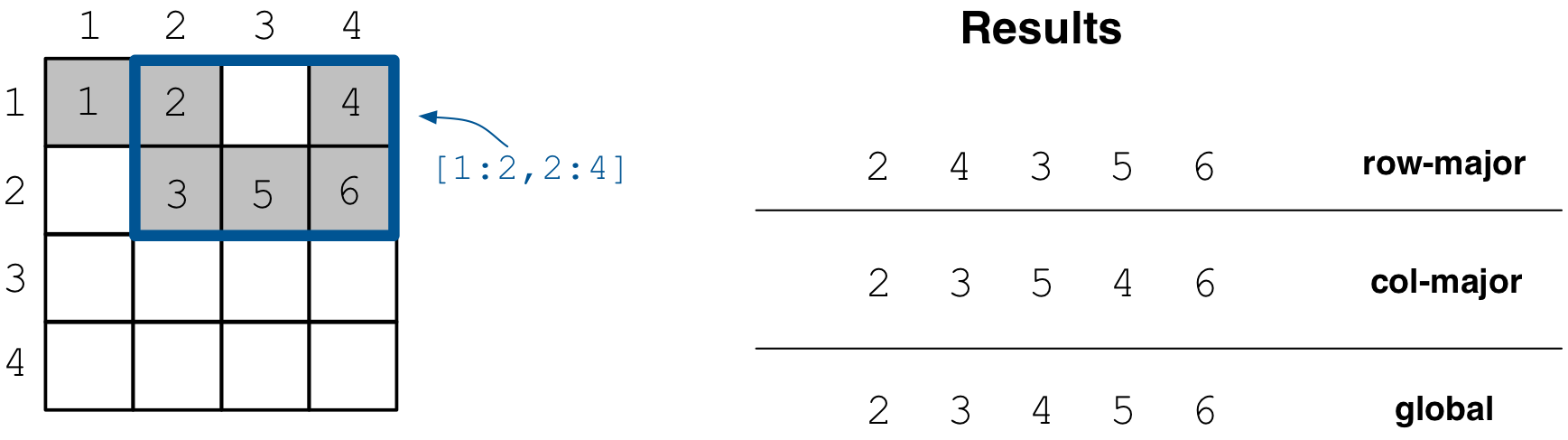
The case of sparse arrays is similar. We use code example reading_sparse_layouts, which creates a 4x4 array with 2x2 space tiling as well. The figure below depicts the contents of the array and the different layouts of the retuned results. The cell values here also imply the global physical cell order.

Running the program, you get the following output.

C++

$ g++ -std=c++11 reading_sparse_layouts.cc -o reading_sparse_layouts_cpp -ltiledb
$ ./reading_sparse_layouts_cpp row
Non-empty domain: [1,2], [1,4]
Cell (1, 2) has data 2
Cell (1, 4) has data 4
Cell (2, 2) has data 3
Cell (2, 3) has data 5
Cell (2, 4) has data 6
$ ./reading_sparse_layouts_cpp col
Non-empty domain: [1,2], [1,4]
Cell (1, 2) has data 2
Cell (2, 2) has data 3
Cell (2, 3) has data 5
Cell (1, 4) has data 4
Cell (2, 4) has data 6
$ ./reading_sparse_layouts_cpp global
Non-empty domain: [1,2], [1,4]
Cell (1, 2) has data 2
Cell (2, 2) has data 3
Cell (1, 4) has data 4
Cell (2, 3) has data 5
Cell (2, 4) has data 6

Python

$ python reading_sparse_layouts.py row
Non-empty domain: ((1, 2), (1, 4))
Cell (1, 2) has data 2
Cell (1, 4) has data 4
Cell (2, 2) has data 3
Cell (2, 3) has data 5
Cell (2, 4) has data 6
$ python reading_sparse_layouts.py col
Non-empty domain: ((1, 2), (1, 4))
Cell (1, 2) has data 2
Cell (2, 2) has data 3
Cell (2, 3) has data 5
Cell (1, 4) has data 4
Cell (2, 4) has data 6
$ python reading_sparse_layouts.py global
Non-empty domain: ((1, 2), (1, 4))
Cell (1, 2) has data 2
Cell (2, 2) has data 3
Cell (1, 4) has data 4
Cell (2, 3) has data 5
Cell (2, 4) has data 6

Allocating the result buffers

Note

The Python API efficiently handles all buffer allocation internally. Therefore, you can skip this section if you are using the Python API.

Recall how the read queries work in TileDB: you allocate the buffers that will hold the results, you set the buffers to the query object (for each attribute), you submit the query, and TileDB populates your buffers with the query results. In other words, memory management falls entirely on you. This is because TileDB was designed for maximum performance (especially when it is being integrated with high-level languages such as Python); this approach minimizes the amount of copying that happens internally.

For dense arrays with fixed attributes, it is fairly easy to calculate how much space you need for your results. This is because you know your subarray and you know that dense reads return a result for every cell contained in the subarray (even for empty cells).

However, it is extremely challenging to accurately calculate how much space you need when you have variable-length attributes (in both dense and sparse arrays), or when you read sparse arrays. For variable-length attributes, even if you know how many cells your subarray contains, you cannot know how much space each cell requires to store an a priori unknown variable-length value. For sparse arrays, you cannot know a priori how many cells in your subarray are empty and non-empty (recall that sparse array reads return values only for the non-empty cells).

To mitigate this problem, TileDB offers some very useful functions. First, it allows you to calculate a good upper bound estimate on the buffer sizes needed to store the entire result for each attribute. If you allocate your buffers based on those estimates, you are guaranteed to get your results without any buffer overflow. We did that in the above sparse example as follows:

C++

auto max_el = array.max_buffer_elements(subarray);
std::vector<int> data(max_el["a"].second);
std::vector<int> coords(max_el[TILEDB_COORDS].second);

Note that these upper bounds are estimates. You should be very careful since, especially when your array has many fragments, they may be quite large. You should always check to see if the returned sizes are “acceptable” for your application prior to allocating the result buffers.

Moreover, since these maximum buffer sizes do not accurately tell you what your result size is, how can you know how many results your query returned? You can get this information from another useful function as follows:

C++

auto result_num = (int)query.result_buffer_elements()["a"].second;

Note the above function tells you how many “useful” elements your query retrieved for each attribute. Since attribute a above is a fixed-length attribute storing a single integer value, it happens that this is equivalent to the number of results. If a stored two integers in each cell, you would have to divide the above number with 2. If we wanted to get the number of results from the coordinates attribute, we would have to write the following instead, since each coordinate tuple for a cell in our 2D example consists of two values:

C++

auto result_num = (int)query.result_buffer_elements()[TILEDB_COORDS].second / 2;

For a detailed description of how to parse variable-length results using the above function, see Variable-length Attributes.

Getting the non-empty domain

We have shown in earlier tutorials that you can populate only parts of a dense array, whereas sparse arrays (by definition) have empty cells. TileDB offers an auxialiary function for calculating the non-empty domain. Specifically, the non-empty domain in TileDB is the tightest hyper-rectangle that contains all the non-empty cells. We retrieved the non-empty domain in the above examples as follows:

C++

auto non_empty_domain = array.non_empty_domain<int>();
std::cout << "Non-empty domain: ";
std::cout << "[" << non_empty_domain[0].second.first << ","
          << non_empty_domain[0].second.second << "], ["
          << non_empty_domain[1].second.first << ","
          << non_empty_domain[1].second.second << "]\n";

Python

print("Non-empty domain: {}".format(A.nonempty_domain()))

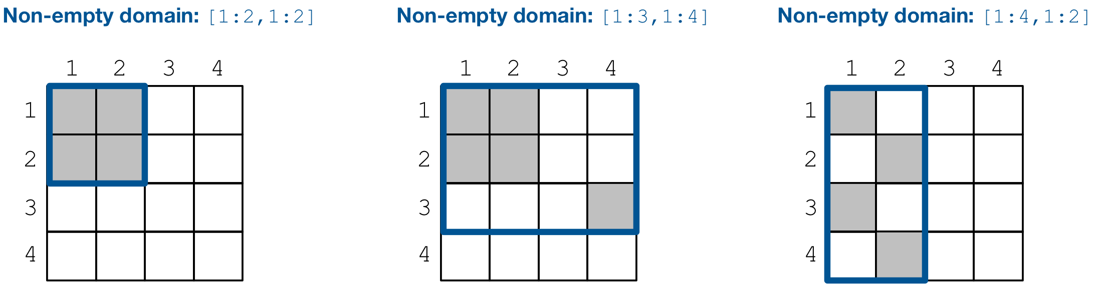
For the dense array example the non-empty domain is [1,4], [1,4], whereas for the sparse one it is [1,2], [1,4]. Note that the non-empty domain does not imply that every cell therein is non-empty. In contrast, it guarantees that every cell outside the non-empty domain is empty. The concept of the non-empty domain is equivalent in both dense and sparse arrays. The figure below illustrates the non-empty domain in some more array examples (non-empty cells are depicted in grey).

Incomplete queries

Warning

Currently incomplete query handling is not supported in the Python API.

There are scenarios where you may have a specific memory budget for your result buffers. As explained above, TileDB allows you to get an upper bound on the result sizes for your desired subarray query, which is particularly useful for variable-length attributes and sparse arrays. But what if the maximum buffer sizes are larger than your memory budget? In this case, you would have to split your subarray manually and try to find query partitions, such that the maximum buffer sizes for each partition are not larger than your memory budget. This can prove extremely cumbersome. Moreover, since the upper bound is an estimate, there may be cases where the maximum buffer sizes are larger than your memory budget, even for very small subarrays.

To address the above issue, TileDB offers an exciting feature. You can allocate any (non-zero) size to your buffers when setting them to your query. If the result size is larger than your buffers can accommodate, instead of crashing, TileDB will gracefully terminate with an incomplete status that you can check. More interestingly, TileDB will attempt to fill as many results as it can in your buffers, and record some internal state that will allow it to resume in the next submission. TileDB is smart enough to continue from where it left off, without sacrificing performance by retrieving again the already reported results.

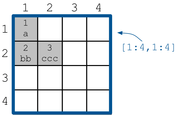
We demonstrate this feature with code example reading_incomplete, which creates a very simple sparse array with two attributes, an integer and a string. The figure below shows the array contents on both attributes.

Below we show our read function. The first observation is that we do not allocate enough space to our buffers to hold the entire result (and we do not use the auxiliary function to get the maximum buffer sizes as we did before).

C++

void read_array() {
  Context ctx;
  Array array(ctx, array_name, TILEDB_READ);
  const std::vector<int> subarray = {1, 4, 1, 4};

  // Prepare buffers such that the results **cannot** fit
  std::vector<int> coords(2);
  std::vector<int> a1_data(1);
  std::vector<uint64_t> a2_off(1);
  std::string a2_data;
  a2_data.resize(1);

  // Prepare the query
  Query query(ctx, array);
  query.set_subarray(subarray)
       .set_layout(TILEDB_ROW_MAJOR)
       .set_buffer("a1", a1_data)
       .set_buffer("a2", a2_off, a2_data)
       .set_coordinates(coords);

  // Create a loop
  Query::Status status;
  do {
    query.submit();
    status = query.query_status();

    // If any results were retrieved, parse and print them
    auto result_num = (int)query.result_buffer_elements()["a1"].second;
    if (status == Query::Status::INCOMPLETE && result_num == 0) {  // VERY IMPORTANT!!
      reallocate_buffers(&coords, &a1_data, &a2_off, &a2_data);
      query.set_buffer("a1", a1_data)
           .set_buffer("a2", a2_off, a2_data)
           .set_coordinates(coords);
    } else if (result_num > 0) {
      print_results(coords, a1_data, a2_off, a2_data, query.result_buffer_elements());
    }
  } while (status == Query::Status::INCOMPLETE);

  // Handle error
  if (status == Query::Status::FAILED) {
    std::cout << "Error in reading\n";
    return;
  }

  // Close the array
  array.close();
}

The second observation is that we keep on submitting the query in a loop. Immediately after the query submission, we retrieve the query status, we print any retrieved results, and then we continue the loop for as long as the query is incomplete. The results that we print in each iteration are always newly retrieved results. In other words, this loop simulates an iterator. At some point, we retrieve all the results, the query becomes completed and the loop terminates.

Let us inspect the output after compiling and running the program.

$ g++ -std=c++11 reading_incomplete.cc -o reading_incomplete_cpp -ltiledb
$ ./reading_incomplete_cpp
Printing results...
Cell (1, 1), a1: 1, a2: a
Reallocating...
Printing results...
Cell (2, 1), a1: 2, a2: bb
Reallocating...
Printing results...
Cell (2, 2), a1: 3, a2: ccc

Each time Printing results... is printed, a new query submission has occurred and new results have been retrieved, which are printed immediately after. Similar to what we have explained above and in tutorial Variable-length Attributes, we can parse the results using the number of result elements returned by query.result_buffer_elements. Note that the results are “synchronized” across attributes: the query returns the same number of result cell values for each attribute, in order to facilitate tracking the progress.

Finally, observe that the program prints Reallocating... to the output, suggesting that function reallocate_buffers was called in the loop. There are cases where the query is incomplete and has not returned any result. This is an indication that the current buffer sizes cannot accommodate even a single result. You must handle these cases with extreme care, otherwise you may get an infinite loop. In our example, we choose to reallocate our buffers. Observe that initially we had a string buffer of size 1, therefore the first result was retrieved without reallocation. However, the second result required a larger buffer and therefore reallocation was triggered (increasing the string size to 2). But then the third string result could not fit in the next iteration (because it was of size 3) and therefore reallocation got triggered once again. Note that, after reallocating your buffers, you need to reset them to the query object.

The above example was rather contrived. In the general case and given that your memory budget is reasonable, the above approach will complete quickly and any extra cost stemming from pausing and resuming the query gets amortized over the entire execution.

Multi-range subarrays

So far all the examples involved a single multi-dimensional rectangular range, created by specifying a single 1D range per dimension. TileDB also supports multi-range subarrays, i.e., it allows specifying multiple 1D ranges per dimension. The resulting subarray consists of the cross product of all the 1D ranges across all dimensions.

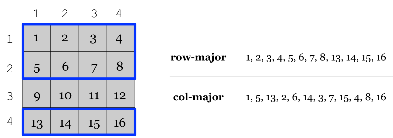
The feature is better illustrated with an example. The figure below illustrates multi-range subarray ([1,2], [4,4]) x [1,4], which slices rows 1, 2, 4 (two ranges along the rows dimension) and columns 1, 2, 3, 4 (one range along the columns dimension). Note above that the 1D row ranges form a list, i.e., their order matters as it dictates the order of the results. For dense arrays, the permissible layouts are row-major and column-major. Note that the global layout is not supported for multi-range subarrays (whereas unordered reads are not supported at all for dense arrays).

Here is how a mult-range read subarray can be specified (from program multi_range_subarray).

C++

void read_array() {
  Context ctx;

  // Prepare the array for reading
  Array array(ctx, array_name, TILEDB_READ);

  // Prepare the vector that will hold the result (of size 6 elements)
  std::vector<int> data(12);

  // Prepare the query
  Query query(ctx, array, TILEDB_READ);
  query.set_layout(TILEDB_ROW_MAJOR).set_buffer("a", data);

  // Add multi-range subarray to query
  int row_0_start = 1, row_0_end = 2;
  int row_1_start = 4, row_1_end = 4;
  int col_0_start = 1, col_0_end = 4;
  query.add_range(0, row_0_start, row_0_end)
      .add_range(0, row_1_start, row_1_end)
      .add_range(1, col_0_start, col_0_end);

  // Submit the query and close the array.
  query.submit();
  array.close();

  // Print out the results.
  for (auto d : data)
    std::cout << d << " ";
  std::cout << "\n";
}

Compiling and running the program we get the following output.

$ g++ -std=c++11 multi_range_subarray.cc -o multi_range_subarray_cpp -ltiledb
$ ./multi_range_subarray_cpp
1 2 3 4 5 6 7 8 13 14 15 16

Multi-range subarrays are applicable to sparse arrays as well and are specified in an identical manner. In addition to row-major and column-major layouts, sparse arrays support also the unordered layout for multi-range subarrays. This layout leads typically to better performance since additional sorting (to respect a particular order) is avoided internally wherever possible.

Furthermore, note that the user may specify ranges with duplicate values, i.e., some of the dimension domain values may be inclued in more than one 1D ranges per dimension. For example, in the example above, the user may issue subarray ([1,2], [4,4], [2,2]) x [1,4], where row 2 appears in two row ranges. In this case, assuming a row-major layout, the results are

1 2 3 4 5 6 7 8 13 14 15 16 5 6 7 8

In general, issuing multi-range subarray queries is faster than submitting the same queries separately as single-range queries. This is because TileDB performs various optimizations internally, such as batching the IO operations and performing them in parallel, avoiding fetching the same tile multiple times if more than one ranges intersect it, etc.

Reading and performance

There are numerous factors affecting the read performance, from the way the arrays were tiled and written, to the number of fragments, to the read query layout, to the level of internal concurrency, and more. See the Introduction to Performance tutorial for more information about the TileDB performance.