Tiling Sparse Arrays¶

In this tutorial you will learn about the core concept of tiling in TileDB, focusing on sparse arrays. It is recommended that you read the previous tutorials on sparse arrays and attributes first, as well as on dense array tiling so that you can better understand the differences from sparse tiling.

Basic concepts and definitions¶

Empty/Non-empty cells

In a sparse array, there are cells that are empty (i.e., they contain no value). TileDB stores only the values of non-empty cells in persistent storage, ignoring the empty cells.

Data tile

The definition of a data tile in sparse arrays is different from that in dense arrays. In this tutorial we will explain that a data tile contains values only from the non-empty cells. Moreover, a data tile does not always correspond to a space tile.

Tile capacity

This is the number of non-empty cells stored in a data tile. We will explain soon that all data tiles in a sparse array have the same capacity, which is specified by the user upon the array creation.

MBR

The minimum bounding rectangle (MBR) of a data tile is a rectangle in the logical view of the array that tightly includes all the non-empty cells whose values are stored in that data tile.

Problem with space tiling¶

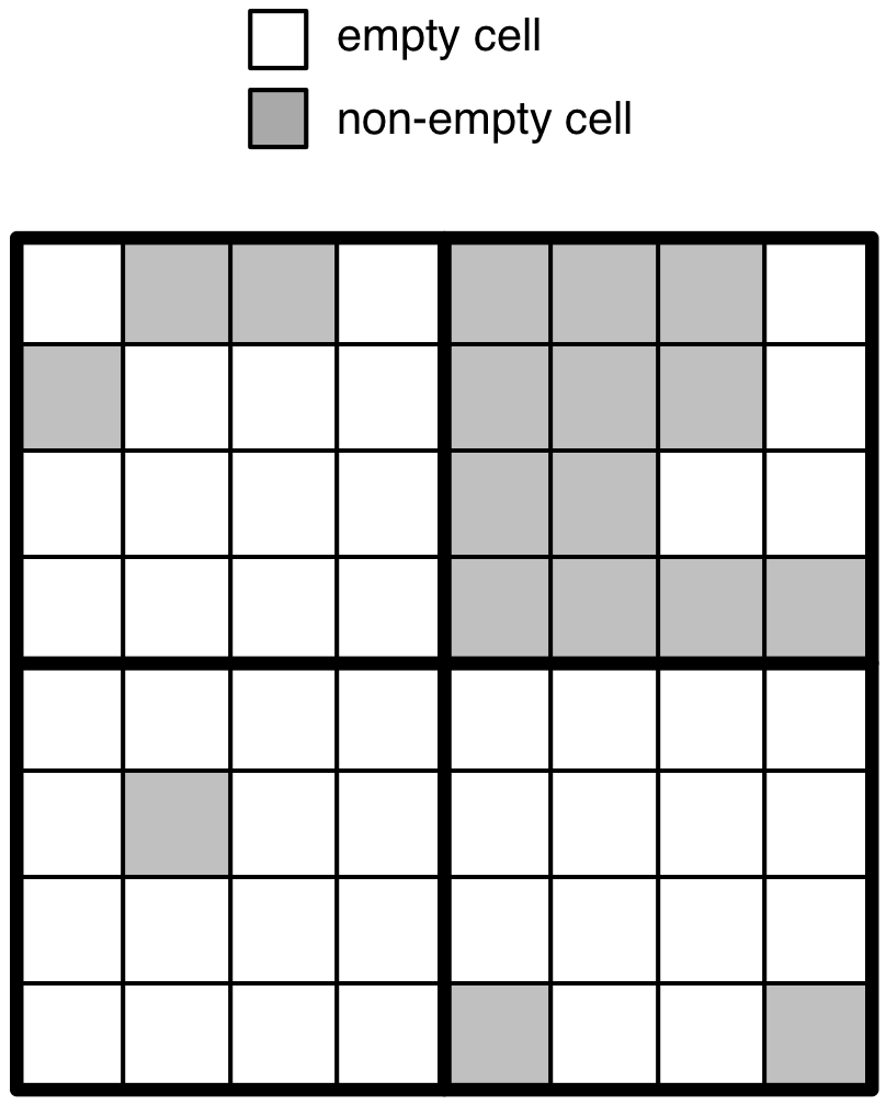
Consider the 8x8 array with 4x4 space tiles in the figure below. Assume for simplicity that the array stores a single (fixed-length) integer attribute. The non-empty (resp. empty) cells are depicted in grey (resp. white) color. If we followed the tiling technique of dense arrays, we would have to create 4 data tiles, one for each space tile. TileDB does not materialize empty cells, i.e., it stores only the values of the non-empty cells in the data files. Therefore, the space tiles would produce 4 data tiles with 3 (upper left), 12 (upper right), 1 (lower left) and 2 (lower right) non-empty cells.

../_images/tiling_sparse_space_tiling_problem.png

Recall that the data tile in TileDB is the atomic unit of IO and filtering. The tile size imbalance that may result from space tiling can lead to ineffective compression (if numerous data tiles contain only a handful of values), and inefficient reads (if the subarray you wish to read only partially intersects with a huge tile, which needs to be fetched in its entirety and potentially decompressed). Ideally, we wish every data tile to store to the same number of non-empty cells. Recall that this is achieved in the dense case by definition, since each space tile has the same shape (equal number of cells) and every data tile contains the values of the cells in a space tile. Finally, since the distribution of the non-empty cells in the array may be arbitrary, it is phenomenally difficult to fine-tune the space tiling in a way that leads to load-balanced data tiles storing an acceptable number of non-empty cells, or even completely unattainable.

Physical cell layout¶

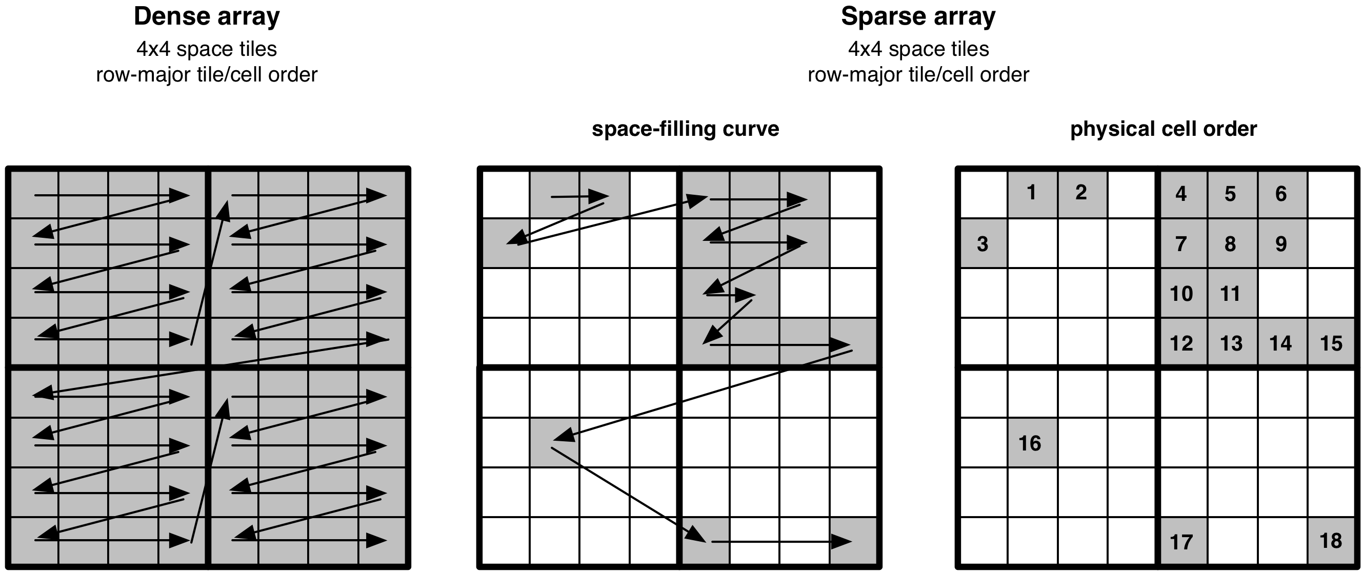
TileDB solves the above, seemingly very challenging, problem in a surprisingly simple manner. Before we explain how TileDB creates the data tiles, we first describe the physical layout of the non-empty cells in sparse arrays, i.e., the global cell order. We focus on this first, because we already know how to do it:

Note

The global order of the non-empty cells in a sparse array is equivalent to that in a dense array, ignoring the empty cells.

The figure below demonstrates the physical cell layout in sparse arrays, and its connection to the layout in dense arrays. Note that, similar to the dense case, the user is the one dictating the global cell order, by specifying the space tiles (i.e., tile extents) and tile/cell order upon array creation.

../_images/tiling_sparse_physical_cell_layout.png

Tiling a sparse array¶

We have two facts so far:

We know how to define a global cell order (and we are quite flexible about it)
We must address the data tile imbalance we explained above.

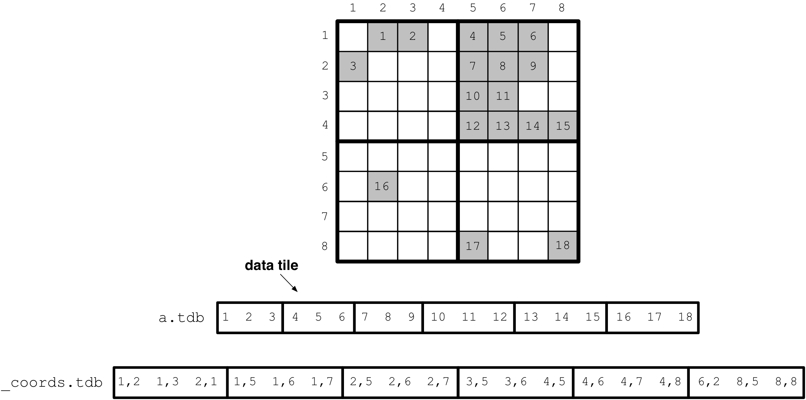
All we need to do is specify the fixed number of non-empty cells we would like each data tile to correspond to. We call this the tile capacity. By specifying the tile capacity, we are instructing TileDB to chunk the already sorted non-empty cells (on the global order) into data tiles of equal cardinality. Continuing the example above, supposing that the non-empty cells contain integers 1-18 that happen to follow the global order (for simplicity), and setting the tile capacity to 3, the following figure shows how TileDB creates the data tiles in the attribute file a.tdb. Notice also the extra __coords.tdb file that TileDB creates for storing the coordinates of the non-empty cells. Without this TileDB would not know which cells the values in a.tdb correspond to.

The case of variable-length attributes is similar; a data tile always corresponds to a fixed number of non-empty cells and stores their corresponding values along an attribute. One thing to note though:

Note

The tile capacity specifies the fixed number of non-emtpy cells each data tile should correspond to. This implies that all the data tiles of a fixed-length attribute have the same size in bytes. However, the data tiles of a variable-length attribute may have variable size in bytes, although they have the same capacity.

You can easily specify the tile capacity in the array schema upon array creation as shown below.

C++

schema.set_capacity(3);

Python

schema = tiledb.ArraySchema(..., capacity=3, ...)

Note

The total number of non-empty cells does not need to be divisible by the tile capacity. It is ok for the very last data tile to be contain fewer values than the tile capacity specifies.

Minimum bounding rectangle (MBR)¶

We now know how to create data tiles. But how can TileDB process a subarray query? In the dense case, the space tiling and the fact that every cell contains a value allows TileDB to do some easy internal calculations and efficiently determine which cell values should be reported as results. However, in the sparse case, given a subarray query and no extra information, TileDB would have to probe the __coords.tdb file and see which coordinates fall in the subarray, and then access the corresponding values in a.tdb for the qualifying cells. This can be very inefficient (it may even result in a complete scan of __coords.tdb).

Fortunately, TileDB employs a simple indexing technique. Upon ingestion of the data and when chunking the (sorted) coordinates into data tiles, TileDB creates a minimum bounding rectangle (MBR), i.e., a hyper-rectangle that tightly encompasses the coordinates in each data tile. For our running example, the MBRs of the data tiles are depicted in different colors in the figure below.

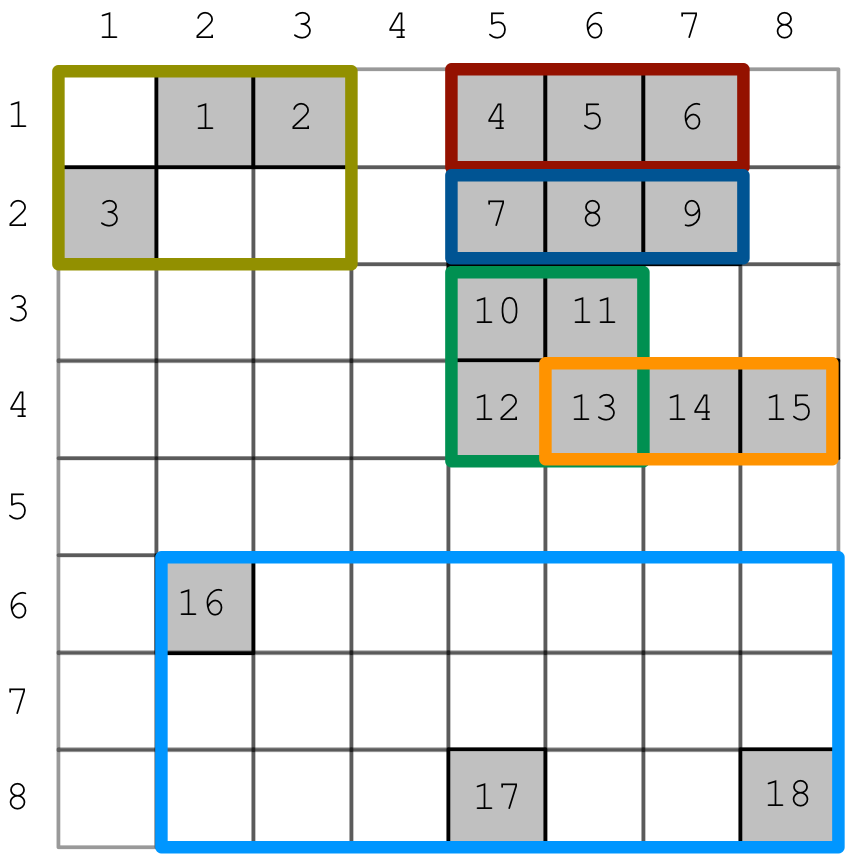
Notice in the figure that 2 MBRs overlap (the green and the orange). In general, the following holds about MBRs.

Note

MBRs are allowed to overlap in TileDB. However, the sets of non-empty cells corresponding to the MBRs are disjoint; each non-empty cell is associated with exactly one MBR. Moreover, the MBRs are allowed to span over multiple space tiles.

The MBRs constitute compact information that is stored in a special __fragment_metadata.tdb file. The MBRs are loaded in main-memory the first time the array is opened (we explain this in later tutorials), i.e., prepared for reading. TileDB uses the MBRs to prune data tiles that certainly do not contain any result, and focuses only on the data tiles whose MBRs intersect with the subarray query. TileDB still needs to probe the overlapping data tiles to discard any coordinates falling outside the subarray (the MBRs are an approximation after all), but this technique significantly boosts the overall read performance.

As a final remark, for readers familiar with spatial indexing, this MBR indexing technique of TileDB adopts ideas from R-Trees.

Space vs. data tiles vs. MBRs¶

We have explained space tiles, data tiles and MBRs, but this may be too much terminology to digest. Let us summarize here these definitions for sparse arrays and provide some more clarifications.

The space tiles simply shape the physical cell layout, i.e., they take part in determining the global cell order. The data tiles are chunks of non-empty cell values in the attribute files with a fixed capacity, similar to the dense case, but (i) they store only values of non-empty cells, and (ii) they do not correspond to space tiles. The MBRs are rectangles that encompass the non-empty cells corresponding to a data tile. There is a one-to-one correspondence between an MBR and a data tile (across all attributes). The MBRs constitute indexing information leading to fast reads.

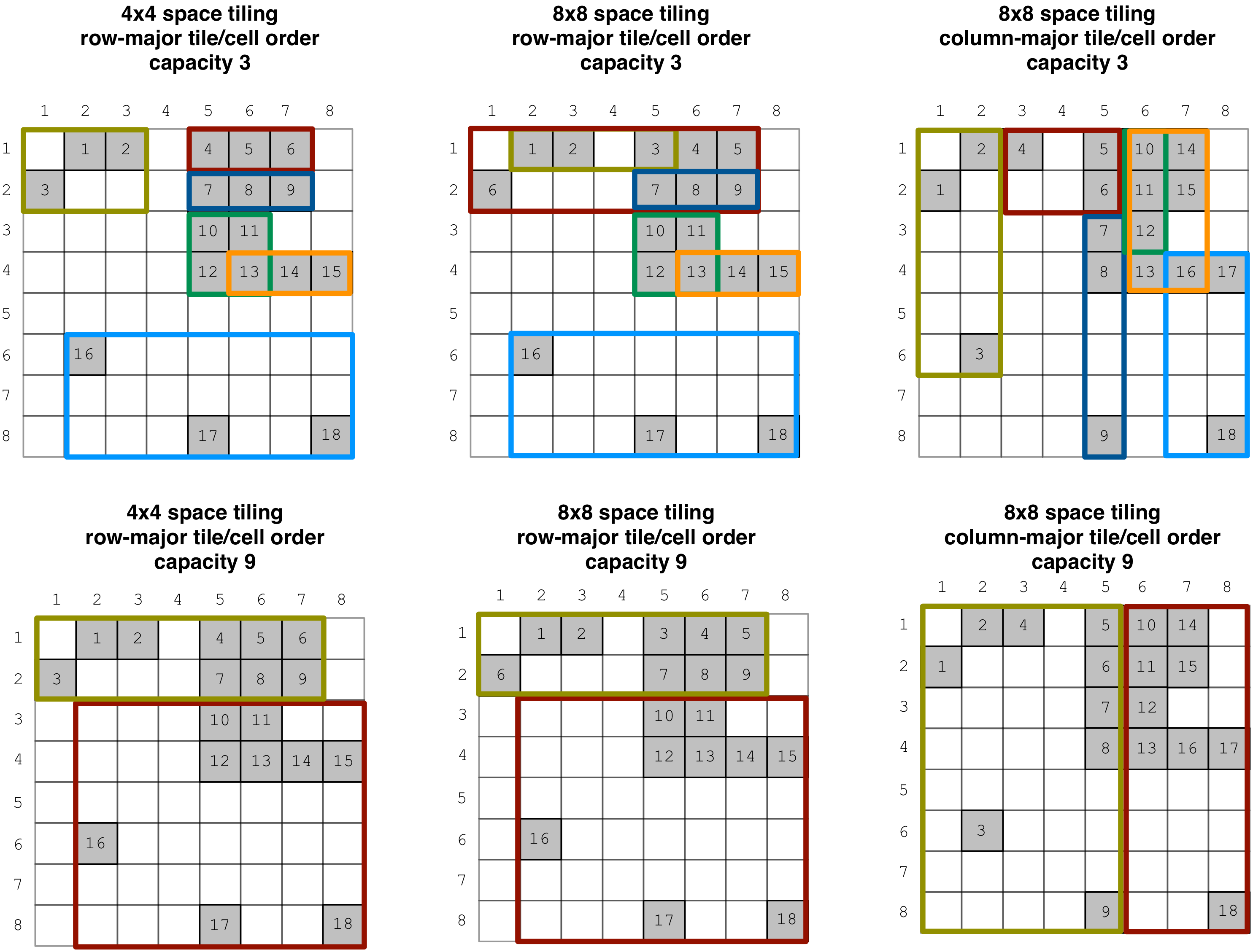
Finally, in case you have not guessed it already, the global order (i.e., the space tiles and tile/cell order) and capacity affect the shape of the MBRs. The figure below demonstrates what happens to the MBRs when varying those parameters (the numbering in the cells follows the global order in each case).

Domain expansion¶

What you know already from dense arrays about domain expansion (which happens when the tile extent along some dimension does not divide the dimension domain) holds also in the case of sparse arrays. However, there is no need for padding tiles with dummy values here. Remember, the data tiles in sparse arrays contain values only for non-empty cells. The only thing you need to be aware of is that domain expansion will happen internally, so you need to make sure that the domain you specify will not exceed the data type bounds after expansion.

Tiling and performance¶

By now you must know that MBRs facilitate reads, as only data tiles with MBRs overlapping a query subarray will be fetched from the files. Moreover, you know that the space tiling, tile/cell order and capacity all affect the shape of the MBRs. Therefore, it is crucial to get these parameters right so that you maximize the TileDB performance for your application. See Introduction to Performance for more details on TileDB performance and how to tune it.