Tiling Dense Arrays

In this tutorial you will learn about the core concept of tiling in TileDB, focusing on dense arrays. It is recommended that you read the previous tutorials on dense arrays and attributes first.

Basic concepts and definitions

Space tile

A space tile is a hyper-rectangular subarray (i.e., array slice) that groups a set of array cells. A dense TileDB array is decomposed into a set of space tiles, each of which having the same shape. The space tiles are defined by the user at the time of array creation, and TileDB stores the tiling information in the array schema.

Tile extent

This is the size of the space tile along some dimension. A space tile can have a different extent on each dimension. All space tiles will have the same tile extents on the same dimension, i.e., all space tiles will have the same shape.

Data tile

A data tile is a group of cell values on a specific attribute. In dense TileDB arrays, for each space tile, there is a corresponding data tile per attribute that stores the values of the cells on this attribute contained in the space tile. A data tile is the atomic unit of I/O and filtering.

Tile order

The tile order or layout (we use these terms interchangeably) is the order of the space tiles, which is defined by the user upon array creation and is stored in the array schema.

Cell order

The cell order or layout (we use these terms interchangeably) is the order of the cells in a space tile, which is defined by the user upon array creation and is stored in the array schema.

Global cell order

The global cell order or layout (we use these terms interchangeably) is the total order imposed on the array cells by the tile and cell order. It determines the way the cell values are physically stored in the TileDB files.

Motivation behind tiling

TileDB is designed to manage massive quantities of data. A large array may not fit in main memory. Therefore, any array access must be performed in chunks of data. Moreover, compresssion is vital in terms of both performance (since heavily compressed data may be transferred faster from the disk or the network into main memory than uncompressed data) and cost (e.g., if the data is stored on some pay-as-you-go service, such as AWS EBS or S3).

To clarify the rationale behind tiling, suppose we create a dense 1Mx1M array with an integer attribute a as follows. The following code defines the array without tiling. In uncompressed form, the cell data consume about 1 TB, whereas suppose for the sake of demonstration that the compressed array consumes 10 GB.

C++

domain.add_dimension(Dimension::create<int>(ctx, "rows", {{1, 1000000}}, 1000000))
      .add_dimension(Dimension::create<int>(ctx, "cols", {{1, 1000000}}, 1000000));
ArraySchema schema(ctx, TILEDB_DENSE);
schema.set_domain(domain).set_order({{TILEDB_ROW_MAJOR, TILEDB_ROW_MAJOR}});
schema.add_attribute(Attribute::create<int>(ctx, "a"));

Python

dom = tiledb.Domain(tiledb.Dim(name="rows", domain=(1, 1000000), tile=1000000, dtype=np.int32),
                    tiledb.Dim(name="cols", domain=(1, 1000000), tile=1000000, dtype=np.int32))
schema = tiledb.ArraySchema(domain=dom, sparse=False,
                            cell_order='row-major', tile_order='row-major',
                            attrs=[tiledb.Attr(name="a", dtype=np.int32)])
tiledb.DenseArray.create(array_name, schema)

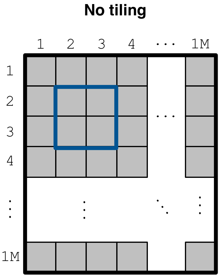
Now suppose we wish to read a tiny 2x2 subarray from this large array as shown in the figure below. Recall that the cell values of this array are written in a file a.tdb inside a subdirectory of the array directory. Suppose that we trivially compress this file (e.g., using any compression tool, such as gzip). In order to retrieve the 2x2 subarray, we will have to decompress the entire file, i.e., to get 16 bytes of data, we will have to fetch and decompress 10 GB of data. Even if we do not compress the file, reading a subarray should entail bringing chunks of data to main memory, instead of retrieving a cell at a time from the file, since each cell retrieval could then mean an I/O system call to the local filesystem, or an HTTP request to a cloud store (such as AWS S3 or Microsoft Azure). For a larger subarray (e.g., 1000x1000) this would incur prohibitive cost.

Tiling a dense array

To mitigate the above problems, we change just two lines of code from the snippet provided above as follows. Notice that we change the last argument in the dimension constructor.

C++

domain.add_dimension(Dimension::create<int>(ctx, "rows", {{1, 1000000}}, 3))
      .add_dimension(Dimension::create<int>(ctx, "cols", {{1, 1000000}}, 2));

Python

dom = tiledb.Domain(tiledb.Dim(name="rows", domain=(1, 1000000), tile=3, dtype=np.int32),
                    tiledb.Dim(name="cols", domain=(1, 1000000), tile=2, dtype=np.int32))

This means that we define the tile extent for dimension rows to be equal to 3 (this used to be 1000000), and the tile extent for dimension cols to be equal to 2 (this used to be 1000000 as well). This effectively decomposes the array into space tiles, each with shape 3x2. It also instructs TileDB to chunk the cell values in a.tdb, such that each group corresponds to one space tile. Each such chunk, called a data tile, is the atomic unit of I/O and compression. 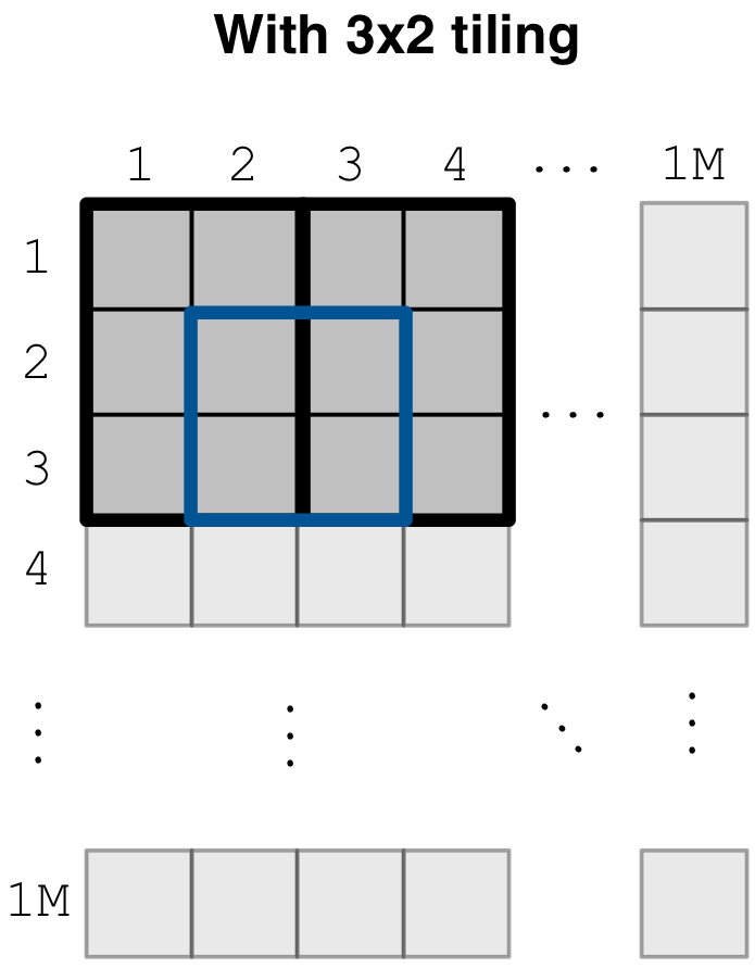This means that (i) if the user specifies compression (to be covered in later tutorials), TileDB will compress each data tile separately, and (ii) entire (compressed or uncompressed) data tiles will always be retrieved from persistent storage, even if we just need to read a single cell value from the tile. The figure below illustrates the same array as above, where each space tile is depicted as a thick black 3x2 rectangle. Now reading the 2x2 subarray (in thick blue) entails fetching the data tiles corresponding to the two overlapping space tiles, ignoring the rest of the array. This significantly reduces the amount of redundant values retrieved when slicing, while allowing compression and efficient I/O.

Physical cell layout

So far we have demonstrated the importance of tiling and how to define space tiles upon array creation. But how do the cell values get physically stored in the data files? Note that an array can be n-dimensional, but the files storing the cell values understand only a single dimension. We later explain that the physical cell layout can greatly affect performance. To answer the above question, we first need to explain the tile order and cell order, and how the user can specify them.

Consider the code line below. Recall that this has been used in all our earlier examples when creating the array schema. This sets both the tile and cell order to row-major (the first element in the pair corresponds to the tile order and the second to the cell order). Another possible order is column-major. Therefore, there are 4 different combinations for setting the tile/cell order, which effectively results in 4 different physical cell layouts (always given a particular space tiling - the combinations increase rapidly as the user is flexible to adjust the tile extents along each dimension).

C++

schema.set_order({{TILEDB_ROW_MAJOR, TILEDB_ROW_MAJOR}});

Python

schema = tiledb.ArraySchema(..., cell_order='row-major', tile_order='row-major', ...)

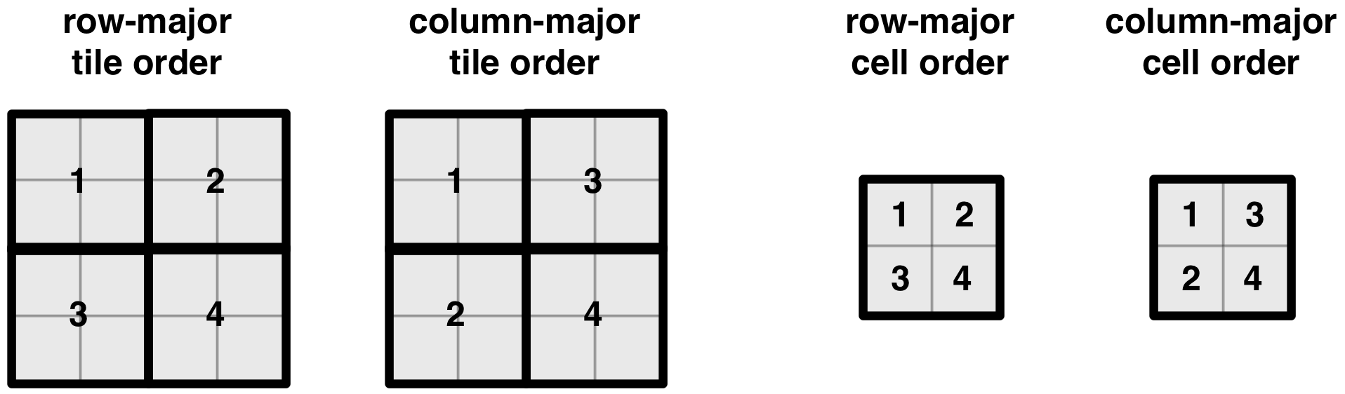
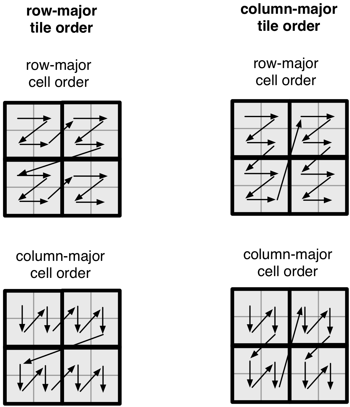
The figure below illustrates the two tile orders and two cell orders for a simple 4x4 array with a 2x2 space tiling. Note that the cell order specifies the layout of the cells inside a space tile.

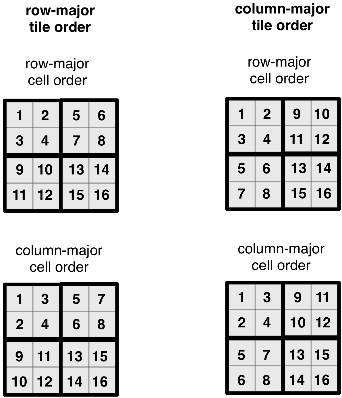
We next demonstrate the effect of a tile/cell order combination on the physical cell layout. The figure below illustrates all four possible cell layouts for the 4x4 array with the 2x2 space tiling. Note that the same cell order applies to all tiles. The numbering of the cells indicates the position where the corresponding cell value is stored in the attribute file (for every attribute).

Observe that the tile and cell order essentially superimpose a space-filling curve on the array, mapping n-dimensional cells to a 1-dimensional order. This is more evident in the figure below.

Note

The physical cell layout, as specified by the space tiling, tile order and cell order upon creating the array schema, is called the global cell order.

Space vs. data tiles

In this subsection we revisit the concepts of space and data tiles in order to clarify and distinguish between these two definitions. Consider the example 4x4 array of the figure below, with a 2x2 tiling and row-major tile and cell order. Suppose also that the array has two attributes; a fixed-length a1 storing integers and a variable-length a2 storing strings. The figure depicts the logical view of the array, as well as its physical view (i.e., the layout of the cell values in the attribute data files) assuming no compression.

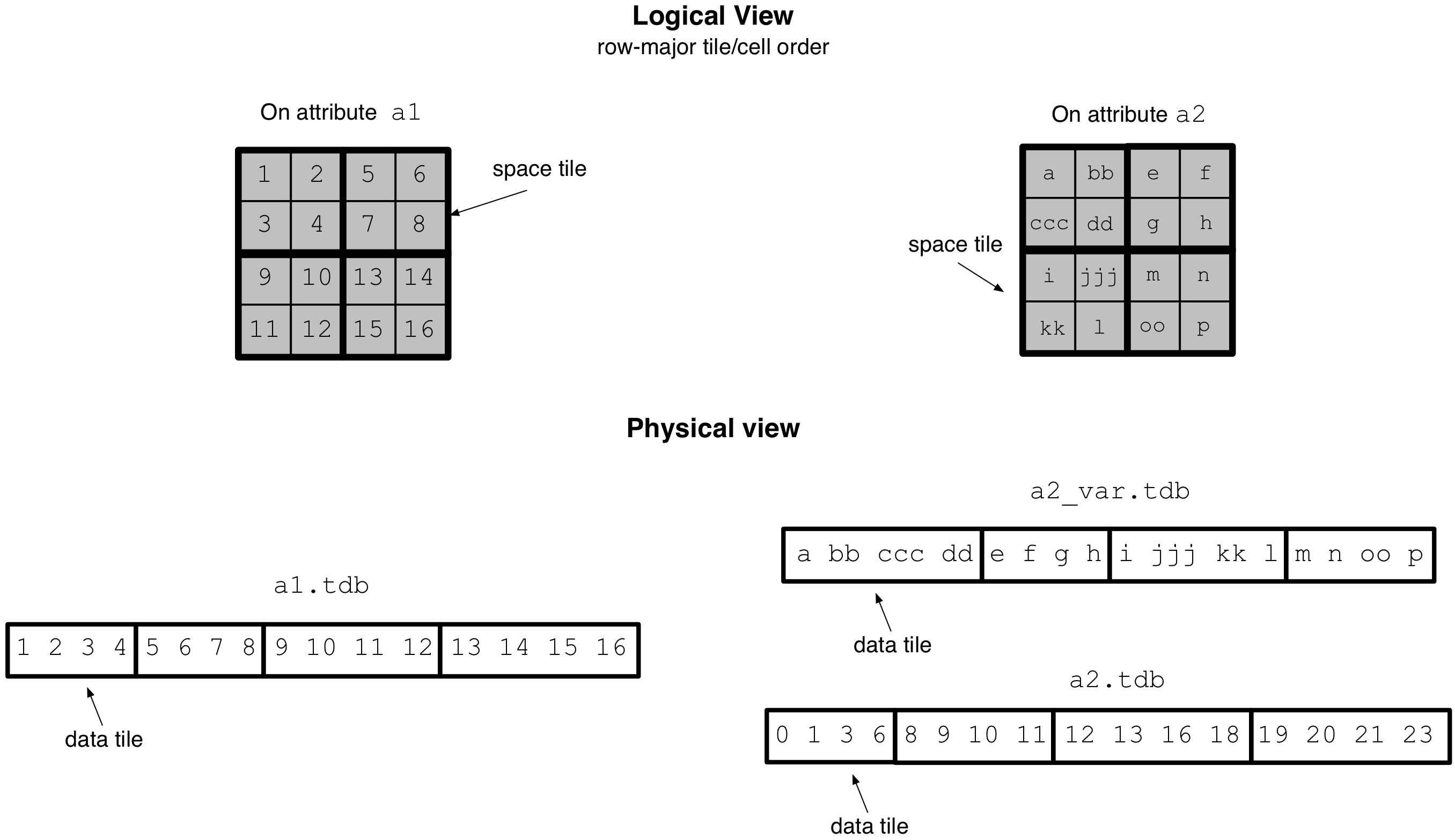
Observe that the space tile is defined in the logical view of the array, whereas a data tile corresponds to a chunk of data in an attribute file, i.e, it is defined in the array physical view. In dense arrays, a data tile always stores the cell values contained in a space tile (in a later tutorial we will see that this may not be true for sparse arrays). Moreover, in the case of variable-length attributes, for each space tile there are two data tiles; the first stores the actual cell values in the space tile along the attribute, and the second stores their corresponding starting offsets in the data file. Finally, observe that the data tiles of a variable-length attribute may have variable physical sizes.

Domain expansion

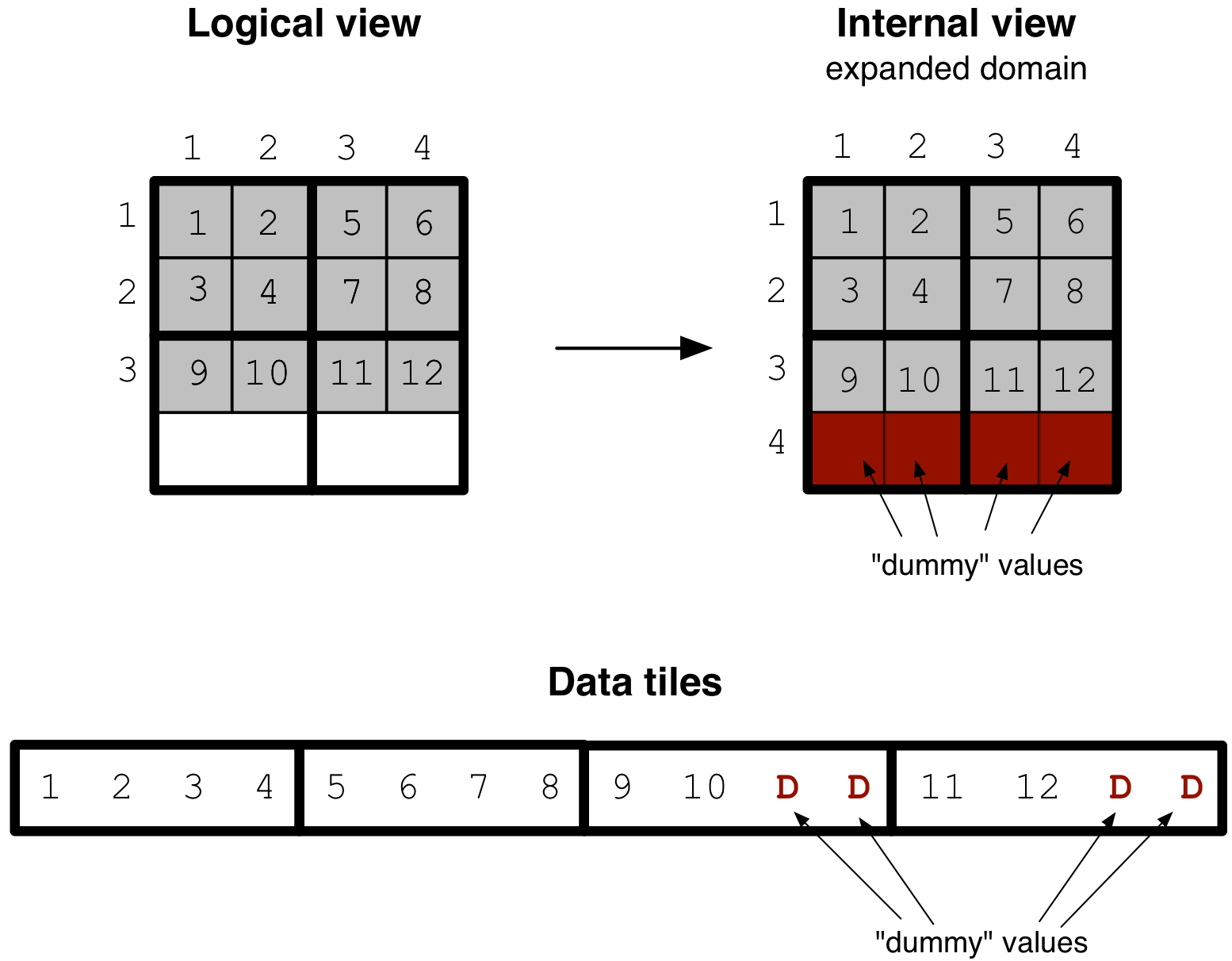
We have stated above that all space tiles in a TileDB array have the same shape. However, what happens in case the array domain cannot be decomposed into integral (i.e., full) space tiles? Consider the following example of a 3x4 array with a 2x2 tiling. Since TileDB cannot handle “partial” space tiles, it internally expands the domain minimally so that it contains integral tiles. The cells in the expanded region of the array are filled internally with empty (dummy) values (along all attributes).

This expansion is generally hidden from the user (as it happens internally). However, there are two scenarios where the user must be aware of the domain expansion. The first is when writing in global cell order. This writing mode is explained thoroughly in a later tutorial. The second is when the user specifies a very large domain, highlighted in the following warning.

Warning

When specifying an array domain that cannot be decomposed into integral tiles (i.e., some dimension domain is not divisible by the tile extent along that dimension), always account for the domain expansion. Specifically, make sure to define the dimension domain such that expanding by one tile extent does not lead to a domain bound overflow (for the selected domain data type).

Tiling and performance

Choosing the space tile shape and tile/cell order is a challenging task. The takeaway from this section is that these choices affect the layout of the cell values in the data files, which in turn greatly affect performance depending on the shapes and positions of the subarrays upon reading. See Introduction to Performance for more details on TileDB performance and how to tune it.